••
Stagflation Explained: Why High Inflation and Slow Growth Can Hit at the Same Time
Stagflation combines persistent inflation with weak economic growth and a softer labor market. This guide explains why it happens, how current 2026 conditions compare with the 1970s, and why stagflation creates a difficult policy trade-off for the Federal Reserve.
Share Article:
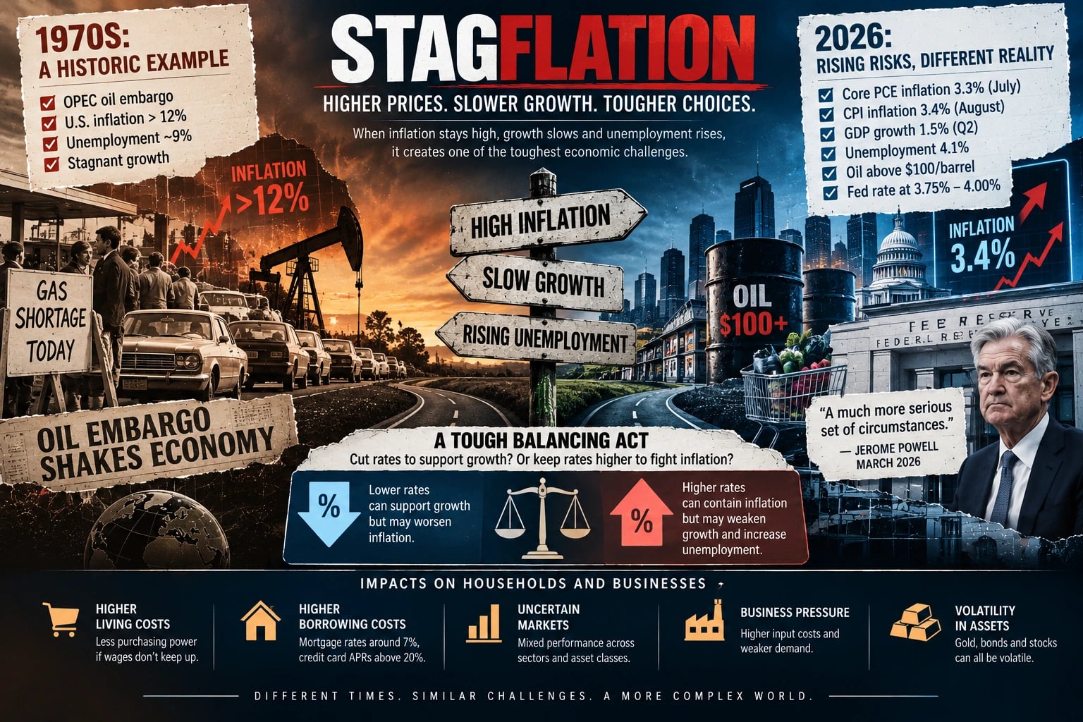
Stagflation is the combination of high inflation, weak or stagnant economic growth, and rising unemployment. It creates an unusually difficult policy environment because the tools used to fight inflation can weaken growth, while measures designed to support growth can add to price pressures. The term became closely associated with the 1970s, when U.S. inflation moved above 12% and unemployment eventually reached 9%.
The issue has returned to economic debate in 2026. Inflation remains above the Federal Reserve's 2% target while economic growth has cooled from earlier highs. The United States is not experiencing a repeat of 1970s-style stagflation, but the combination of sticky prices, slower growth, and energy-market disruption has increased concern about stagflationary risks.
Why Inflation and Stagnation Can Coexist
Traditional discussions of the Phillips curve emphasize a short-run trade-off between inflation and unemployment. When the economy runs hot, unemployment can fall while inflation rises. When activity weakens, price pressure often eases.
Stagflation complicates that relationship because inflation can remain elevated even while economic activity slows.
A major negative supply shock is one way this can happen. If the price of an essential input such as energy rises sharply, businesses face higher costs at the same time households lose purchasing power. Inflation can rise even as demand and output weaken.
The Federal Reserve Bank of Cleveland describes stagflation as unusual because high inflation more commonly occurs during periods of stronger economic activity.
The 1970s provided the best-known example. The OPEC oil embargo sent energy prices sharply higher and increased costs across the economy while growth weakened. Inflation and unemployment rose together, challenging the policy assumptions that had guided much of the postwar period.
The Role of Expectations
Supply shocks can start a stagflationary episode. Expectations can help determine whether it persists.
Kellogg economist Phillip Braun has argued that the 1970s episode cannot be explained by oil shocks alone. Monetary policy also played an important role. Policymakers were reluctant to tighten aggressively while growth was weakening, allowing inflation expectations to become more deeply embedded.
Workers sought higher wages to compensate for rising prices, while businesses faced pressure to pass higher labor and input costs on to consumers.
Once inflation expectations become persistent, reversing them can be economically painful. Under Federal Reserve Chair Paul Volcker, short-term interest rates eventually approached 20% in the early 1980s as the central bank moved aggressively to bring inflation under control.
The 2026 Backdrop: Inflation Above Target, Growth Cooling
The data in 2026 show why stagflation has returned to the economic discussion, even though current conditions remain far less severe than those of the 1970s.
Core PCE inflation, the Federal Reserve's preferred underlying inflation measure, was 3.3% year over year in July 2026. That remained well above the Fed's 2% target.
Consumer inflation also remained elevated. U.S. CPI inflation was 3.4% year over year in August 2026.
Growth, meanwhile, has moderated. Real U.S. GDP increased at a 1.5% annualized rate in the second quarter of 2026. That followed a sharp slowdown at the end of 2025, when the final estimate showed fourth-quarter real GDP growing at only 0.5% annualized.
The labor market remains more resilient than in a traditional stagflation crisis. The unemployment rate was 4.1% in August 2026.
Earlier in the year, February payrolls fell by 92,000 and the unemployment rate stood at 4.4%, highlighting how uneven the labor-market picture has been.
RBC Economics has used the phrase "stagflation lite" to describe an environment where inflation remains stubborn while economic growth struggles to regain stronger momentum.
The Middle East conflict added another source of supply pressure during 2026. Oil moved above USD 100 per barrel as energy markets reacted to disruptions and risks surrounding major shipping routes.
S&P Global's April 2026 flash PMI data also showed weakening demand across major developed economies alongside stronger price pressures. New orders across the G4 economies fell below the 50.0 no-change level for the first time since late 2023.
Those conditions resemble some elements of a stagflationary shock, although they do not by themselves establish that the economy is in full stagflation.
How 2026 Differs From the 1970s
The similarities attract attention, but the differences are substantial.
| Factor | 1970s Stagflation | 2026 Environment |
|---|---|---|
| Main supply shock | Major OPEC oil disruptions | Middle East conflict and elevated energy prices |
| Inflation | U.S. inflation exceeded 12% | Core PCE 3.3% in July; CPI 3.4% in August |
| Unemployment | Eventually reached about 9% | 4.1% in August 2026 |
| Economic growth | Severe periods of stagnation and recession | Q2 GDP grew 1.5% annualized |
| Fed policy | Policy credibility weakened before aggressive tightening | Target range at 3.75%–4.00% after September 2026 hike |
| Labor market | Strong wage-price dynamics | Cooling but comparatively resilient |
| Inflation expectations | Became deeply unanchored | Under pressure but not comparable with the 1970s |
Federal Reserve Chair Jerome Powell resisted applying the 1970s stagflation label to the economy earlier in 2026.
In March, he said he would reserve the term for "a much more serious set of circumstances."
That distinction matters. Inflation remains above target, but it is far below the levels reached during the 1970s. Unemployment is also much lower, and the Federal Reserve retains considerably more credibility in its commitment to price stability.
The current situation is better described as an environment of elevated stagflation risk rather than a repeat of the 1970s.
Why the Policy Response Is So Difficult
Stagflation creates conflicting pressures for central banks.
Cutting interest rates can support growth and employment, but easier monetary policy may worsen inflation.
Raising rates can help contain inflation, but tighter borrowing conditions can reduce investment, weaken consumer demand, and increase unemployment.
The Cleveland Fed summarizes the dilemma directly: policies used to address weak growth can intensify inflation, while policies used to restrain inflation can weaken growth.
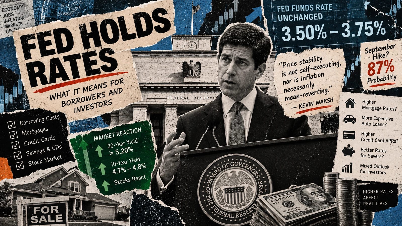
In March 2026, the Federal Reserve held its target range at 3.50%–3.75% as policymakers assessed the effect of energy prices and slowing growth.
Conditions later changed. On September 16, 2026, the Fed raised the federal funds target range by 25 basis points to 3.75%–4.00%, reflecting renewed concern about inflation.
The Fed's dual mandate makes this environment particularly difficult. Policymakers are responsible for both maximum employment and stable prices. When inflation remains high while growth weakens, those goals can pull policy in different directions.
What Stagflation Means for Households and Businesses
The most immediate effect is pressure on purchasing power.
If wages do not rise as quickly as prices, households have less real income available for discretionary spending. Businesses can face weaker demand at the same time their own costs increase.
Walmart reported record fourth-quarter revenue of USD 190.7 billion for fiscal 2026. The company also reported continued strength among higher-income customers, a pattern consistent with consumers increasingly seeking value as household costs remain elevated.
Borrowing costs can also remain high in a stagflationary environment.
The 10-year U.S. Treasury yield crossed 5% on September 14, 2026, its highest level since 2023, before easing to roughly 4.94% on September 17.
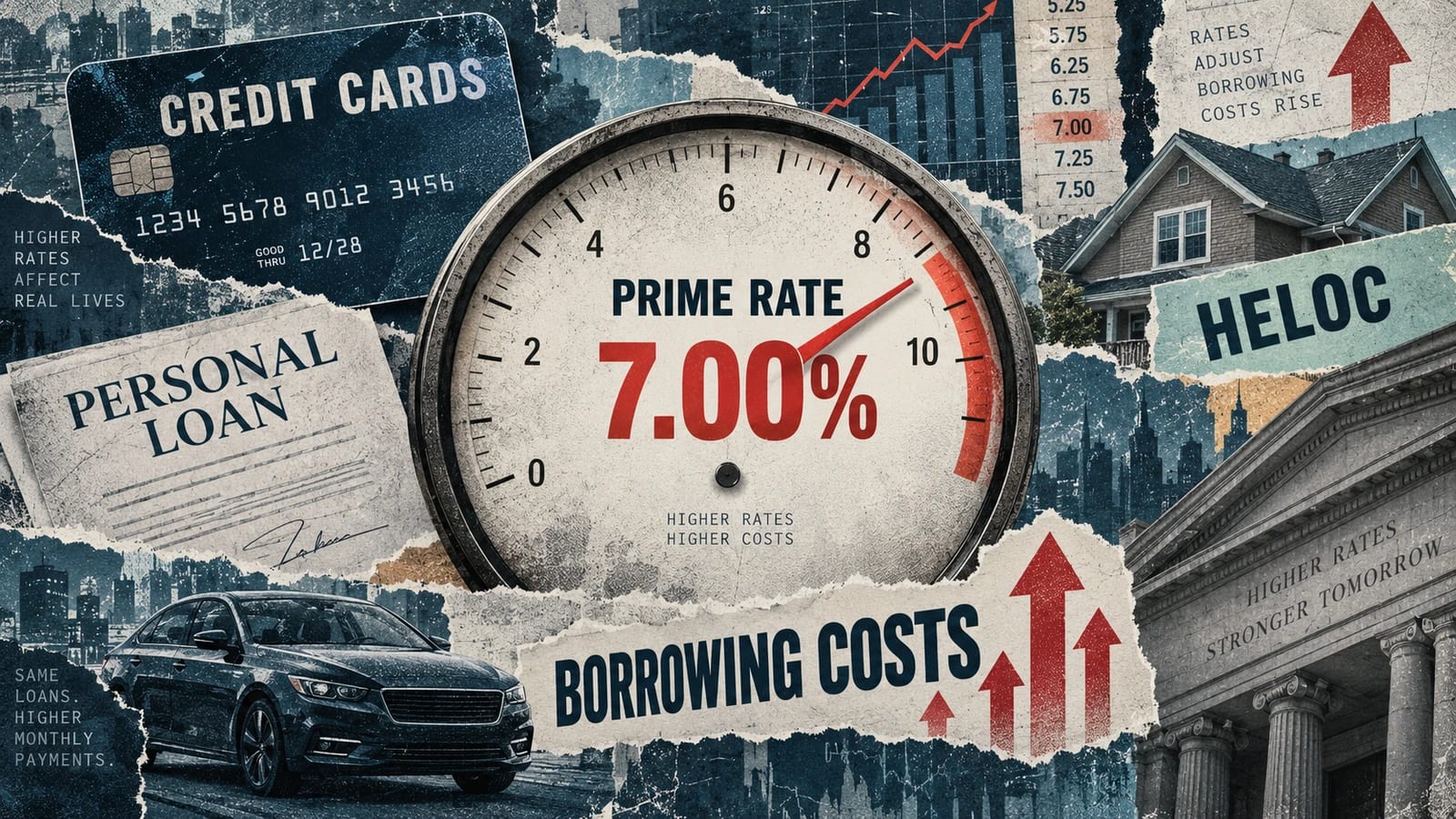
Mortgage rates followed the broader rise in long-term borrowing costs. The average 30-year fixed mortgage rate moved from around 6% in late February to approximately 7% by mid-September.
Credit-card APRs remained above 20% for many borrowers, while the Federal Reserve's September rate increase added further pressure to some variable-rate borrowing costs.
Asset-market performance during stagflationary periods is less predictable than simple rules often suggest.
Higher discount rates can pressure expensive growth stocks, while weaker demand can hurt cyclical industries such as consumer discretionary and industrial companies. Some defensive sectors may prove more resilient, but outcomes depend on valuations, the source of inflation, interest-rate policy, and the duration of the slowdown.
Gold and long-duration bonds can also be volatile. Spot gold traded around USD 4,360 per ounce on September 17, while long-term bond prices reacted sharply to changing inflation and growth expectations.
There is no asset class that performs predictably in every stagflationary episode.
Is the U.S. Actually in Stagflation?
Current data do not support describing the United States as being in a severe 1970s-style stagflation episode.
Inflation remains too high for the Federal Reserve's comfort, but it is nowhere near double-digit levels.
The labor market has cooled, yet unemployment at 4.1% remains far below the levels associated with the 1970s crisis.
Growth is slower, with second-quarter GDP expanding at a 1.5% annualized rate, but the economy is not experiencing the combination of deep stagnation and mass unemployment that defined the historical episode.
The more accurate description is that stagflation risks have increased.
A prolonged energy shock, persistent inflation, weaker consumer demand, and further deterioration in the labor market could make that risk more serious. If energy pressures ease or inflation falls while growth remains positive, the comparison with the 1970s would weaken.
Disclaimer: This article is for informational and educational purposes only and is not personalized financial, investment, tax, or legal advice. Consult a licensed professional for advice specific to your situation.
Frequently Asked Questions
What is the difference between inflation and stagflation?
Inflation describes a broad rise in prices. Stagflation adds another problem: weak economic growth and a deteriorating labor market occurring alongside persistent inflation. That combination is difficult because the policies normally used to support growth can work against efforts to bring prices under control.
What caused stagflation in the 1970s?
The oil shocks were an important trigger, but they were not the whole story. Economists also point to monetary policy, inflation expectations, wage dynamics, and earlier policy decisions. Persistent inflation emerged from several forces reinforcing one another rather than from oil prices alone.
Is the U.S. in stagflation in 2026?
The latest data point to elevated stagflation risk, not a repeat of the 1970s. Core PCE inflation was 3.3% in July, unemployment was 4.1% in August, and real GDP grew at a 1.5% annualized pace in the second quarter. Inflation is above target and growth has cooled, but unemployment and inflation remain far below the extremes of the historical stagflation period.
Why is stagflation so difficult for the Fed?
The same interest-rate tool affects both sides of the problem. Higher rates can reduce inflation pressure but also slow demand and employment. Lower rates can support activity but risk keeping inflation elevated. Stagflation forces policymakers to balance those costs at the same time.
What can households focus on during a stagflationary environment?
Financial resilience matters more than trying to predict short-term market moves. Households may focus on liquidity, debt costs, essential spending, emergency savings, and the effect of variable interest rates on their budgets. The appropriate choices depend on income stability, expenses, debt obligations, and individual financial circumstances.
From the Desk
All Markets →More in Markets
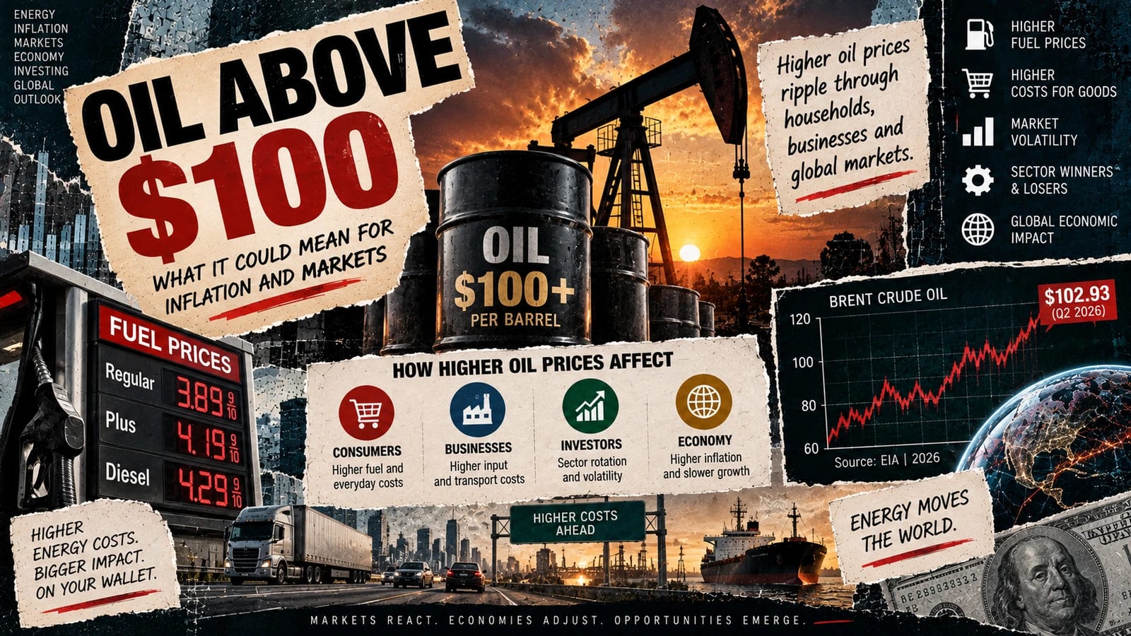
Oil Above 100 USD Inflation Pressures and Market Shifts
Oil above USD 100 per barrel raises inflation, pressures consumer spending, and reshapes sector performance. This guide explains the transmission channels, Fed dilemma, and practical implications.
Fresh Reporting
Browse All Stories →Latest from The Ledger
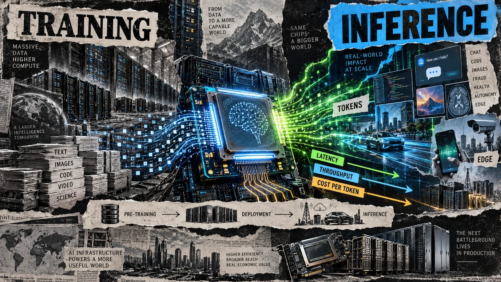
What Is AI Inference? Why the Next AI Chip Battle Is Moving Beyond Training
AI inference is running a trained model to generate outputs on new data. It now accounts for 80% to 90% of AI compute costs and is becoming the main battleground for chipmakers like NVIDIA, AMD, and OpenAI.

Leave a Comment
Your email address will not be published. Required fields are marked *